Mechanistic Interpretability via Layer Patching in a Time-Series Analysis

In the previous posts, I looked at the way GPT-oss classifies astronomical light curves, and especially at the tension between two pieces of information: the timescale of the transient and its color evolution.

The basic task is simple. I give the model two-band photometry (amplitude vs. time), in $g$ and $r$ (corresponding to green and red colors), and ask it to return only one word: TDE or SN. Of course, the actual behavior is not that simple. The model does not just read the light curve and immediately output a class. It generates an internal reasoning sequence, and the final answer appears only after that reasoning has unfolded.

In this post I wanted to ask a more causal question:

If I corrupt one physical feature of the light curve, can I find where in the model this corruption changes the final classification?

To do that, I used activation patching — a standard tool in mechanistic interpretability.

The setup

I started with one light curve that the model classifies as a TDE. Then I created two corrupted versions of the same prompt.

The first corruption changes the time axis. The flux values are kept fixed, but the observation times are compressed. In the clean version, the light curve evolves over tens of days. In the corrupted version, the same flux evolution is presented as happening much faster. This is a classical behavior of the competing class (SN).

The second corruption changes the color evolution after peak. This is motivated by the fact that color is one of the physical features that should help distinguish TDEs from SNe. In a simplified picture, TDEs tend to stay blue for longer, while SNe cool and become redder after peak. In simpler words - for a TDE the green color is always brighter than the red color and for a SN the red color becomes brighter after the peak.

The three light curves are shown in Figure 1.

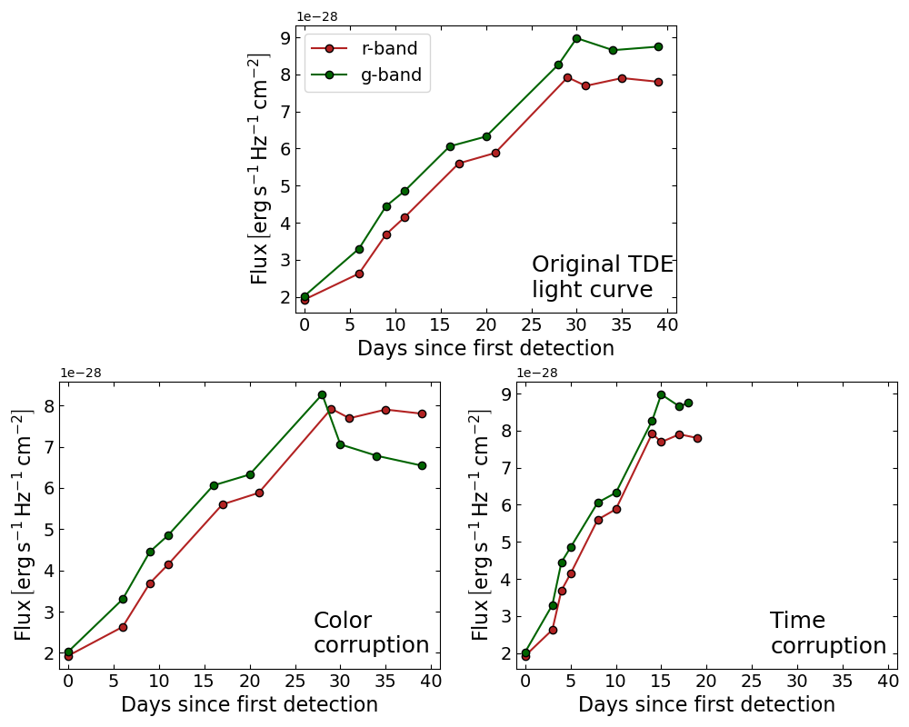
Figure 1. Original light curve (top panel) compared to the two corrupted versions used in this experiment. In the time corruption (bottom right panel), the flux values are kept fixed but the time axis is changed. In the color-after-peak corruption (bottom left panel), the post-peak color evolution is modified while keeping the rest of the prompt structure fixed.

What I patched

The patching experiment is conceptually simple.

First, I run the clean prompt (similar to the one in my previous blog post, with the data from the time-series shown above) through the model and save the hidden states at every layer. Then I run the corrupted prompt, but at one layer at a time I replace the corrupted hidden state with the clean hidden state. I only do this at the last token position.

In other words, for each layer I ask:

If the model sees the corrupted prompt, but at this layer I restore the clean representation at the decision point, does the model move back toward the clean answer?

Technically, this is a corrupted-to-clean patch. The model receives the corrupted sequence, but the residual stream at the last token position is replaced by the clean residual stream at a chosen layer.

Here is the core of the implementation:

@torch.no_grad()
def patch_forward_last_position(model, tokenizer, corrupted_text, clean_cache, layer_idx):
    """
    Run corrupted prefix, but patch the last token hidden state at the output
    of layer `layer_idx` using the clean cache.
    """
    blocks = get_blocks(model)
    inputs = tokenizer(corrupted_text, return_tensors="pt").to(model.device)

    clean_h = clean_cache["hidden_states"][layer_idx + 1][0].to(model.device)
    clean_last = clean_h[-1, :].clone()

    def hook_fn(module, module_input, module_output):
        if isinstance(module_output, tuple):
            hidden = module_output[0].clone()
            hidden[0, -1, :] = clean_last
            return (hidden,) + module_output[1:]
        else:
            hidden = module_output.clone()
            hidden[0, -1, :] = clean_last
            return hidden

    handle = blocks[layer_idx].register_forward_hook(hook_fn)
    try:
        out = model(**inputs, use_cache=False)
    finally:
        handle.remove()

    return out

One important technical point is that the plotted quantity is not literally a probability in the current implementation. I used the first-token log probability difference,

So positive values mean the model is leaning more toward TDE, and negative values mean it is leaning more toward SN.

Time corruption

The first experiment asks whether the model is using the timescale of the light curve. This matters physically. A TDE and a Type Ia SN can both rise and fade, but the timescale is different. If I take a TDE-like flux evolution and make it happen over a much shorter time interval, I am effectively making it look more SN-like, but not entirely as the next section discuss also color evolution (the result is shown in Figure 2).

The key point here is not just whether the final answer changes, but where it changes. Since patching early layers has little effect, but patching a specific range of layers (above Layer 16) causes a strong recovery toward the clean answer, that suggests that the relevant information becomes decision-relevant closer to the surface of the model.

Color-after-peak corruption

The second experiment asks the same question, but for color evolution after peak. This is interesting because in earlier analyses the model often explicitly references timescale more than color. That does not necessarily mean color is unimportant, it might just be used more implicitly or later in the computation. So here I corrupt the color evolution after peak and repeat the same patching experiment (see results in Figure 2).

The comparison between the two lines in Figure 2 is the main point. If both corruptions rise at similar layers, that suggests a shared decision pathway. If they rise at different layers, it suggests that timescale and color enter the decision at different stages.

Interestingly, it seems like they both become important around the same layer! That might means that the model is integrating both features (timescale and color) at the same stage of the computation, rather than processing them in separate, sequential steps. However, this is just a textbook example and we need a better systematic way of testing this hypothesis.

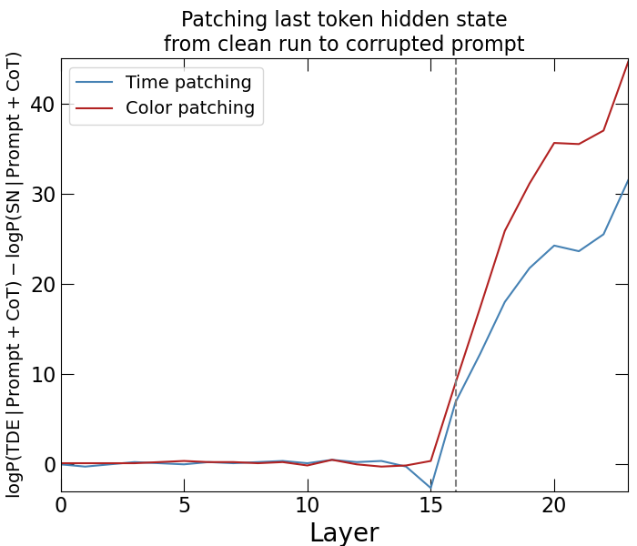
Figure 2. Change in the TDE-vs-SN logit difference as a function of patched layer for the time-corrupted prompt (blue) and color-corrupted prompt (red). Each point corresponds to restoring the clean hidden state at the last token position for one layer.

Closing thoughts and future paths

What I like about this experiment is that it connects the astrophysics and the interpretability in a very direct way. The corruptions are physically motivated: one changes the timescale, and the other changes the color evolution. Then activation patching asks where in the model these features actually matter for the final decision.

This does not prove that the model understands TDEs or SNe in a physical sense. But it does give a controlled way to test whether specific features are causally involved in the classification. A more detailed way to test causality is to patch different token positions, not only the last token. I plan to do it in the future.

For me, this is the useful direction: not only asking whether an LLM can classify a transient, but asking what parts of the input drive that classification, and where in the model those features start to matter. More specifically, I started to think in the following direction: it is obvious that these models does not outperform classical ML approaches and therefore most astrophysicists won’t adopt this approach. On the other hand, using mechanistic interpretability allow us to better understand these model and the decision that they are making and this is a big adventage over other, more traditional, models.

I’ll finish by saying that I didn’t tried SotA models yet, and it is likely that they will do much better (and might even compete with well tested classifiers that are specifically trained for this task). However, I now find the experiment itself much more interesting than achieving better classification scores so I’ve decided to try something new: I am going to clip the model upper layers (making it significantly smaller) and fine tune it for this classification task. If it’ll be successful it can lead to a tool that is not too expensive on the one hand, and super informative on the other. Stay tuned for the results of this experiment!