Bayes’ theorem is probably one of my favorite ideas in statistics. The idea that we update our beliefs based on observed data sits at the core of the scientific method (and should probably be applied for personal interactions, but that is a topic for a different post). Formally, Bayes’ theorem is
\[\mathbb{P}(A \mid B) = \frac{\mathbb{P}(B \mid A) \cdot \mathbb{P}(A)}{\mathbb{P}(B)} ,\]where the posterior, $\mathbb{P}(A \mid B)$, is proportional to the likelihood, $\mathbb{P}(B \mid A)$, times the prior, $\mathbb{P}(A)$.
I think there are aspects of LLM behavior that can be usefully framed in these terms, even if the model is not literally doing textbook Bayesian inference. In this post I focus on two such aspects, using the framework I developed in my recent blog posts:
- Few-shot prompting as a form of prior update through in-context learning
- Sequence-level causal tracing as a way to expose a prior-like bias in the model’s intermediate reasoning
Few-Shot Prompts - updating the model priors?
A common way to improve the performance of an LLM on a specific task is to fine-tune it. But fine-tuning can be expensive, both in computation and in effort. Few-shot prompting (FSP) offers a much cheaper alternative: instead of changing the model weights, we provide a small number of labeled examples in the prompt and let the model adapt in context.
This idea was popularized by Brown et al. (2020) [1], who showed that sufficiently large language models can often improve substantially when given only a handful of demonstrations, in some cases “reaching competitiveness with prior state-of-the-art fine-tuning approaches.”
In my previous blog post, I benchmarked several base LLMs on the task of classifying TDEs and Type Ia SNe. I showed that both GPT-oss base models I tested, the smaller one (20B parameters) and the larger one (120B parameters), do a reasonable job on this classification task, but still underperform relative to a task-specific classifier, namely a specially trained LSTM.
That makes GPT-oss a natural testbed for two prompt-level changes that can be interpreted, loosely, as updating the model’s effective prior:
- Few-shot prompting (FSP): I added two labeled examples before the real dataset. These were “textbook” examples: one clear Type Ia SN and one clear TDE.
- Additional physical context: In my previous post I noticed that the model placed more weight, in its Chain of Thought, on the timescale of the light curve than on the color evolution. To encourage attention to the latter, I added the following line before the actual data:
Take extra care about the color evolution (g-r) before and after peak if it exists. TDEs should be blue (positive g-r) even after peak and SN exhibit cooling after peak, meaning they change from blue (g-r > 0) before peak to red (g-r < 0) after peak.
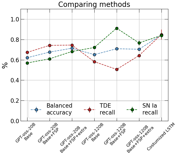
As seen in Figure 1, both of these additions improve the overall balanced accuracy of the GPT-oss models. However, the larger GPT-oss model (120B) shows two somewhat strange behaviors:
- adding FSP increases SN recall while decreasing TDE recall, even though the overall balanced accuracy improves;
- adding extra physical context on top of FSP does not improve the overall balanced accuracy further, although it does reduce some of the bias toward Type Ia SNe.
For the smaller model (20B), the story is cleaner. We see a clear increase in balanced accuracy both when applying FSP and when adding extra physical context. In addition, the model does not overclassify Type Ia SNe as strongly, and the gap between SN recall and TDE recall becomes smaller. If TDE recall is the main quantity of interest, and for me it is, the smaller GPT-oss model actually does quite well, reaching roughly $\sim 70$%.
That said, the specially trained LSTM still outperforms these LLMs. It is also important to note that this comparison is not perfectly apples-to-apples: the LSTM was trained and validated on splits of the dataset, whereas the LLM evaluation here uses the full dataset as an evaluation set. So while the comparison is still informative, it should not be interpreted too literally.
Sequence-Level Causal Tracing - probing the model prior gap?
In the previous section I showed that “updating priors,” at least in an in-context sense, can improve performance. The next question I wanted to ask was: can I actually see a prior-like preference emerge inside the model’s reasoning process?
For that, I used GPT-oss 20B as a case study.
When tracing the model’s Chain of Thought, I noticed two structural features of the generated sequence:
- Before producing the reasoning, the model emits the prefix
"<|channel|>analysis<|message|>",
after which the actual “thinking” begins. - Before producing the final answer, the model emits the prefix
"<|end|><|start|>assistant<|channel|>final<|message|>",
which I refer to asFINAL_HDR.
Using this structure, I first ran a full forward pass for one representative object, a textbook TDE light curve, and generated the full sequence: CoT + FINAL_HDR + final classification.
Then, iteratively, I created modified prefixes consisting of:
- the prompt,
- a partial Chain of Thought,
- and then an early insertion of
FINAL_HDRevery five tokens.
In other words, I forced the model to produce an answer at different stages of its own reasoning process. Conceptually, the intervention asks:
“If you had to decide right now, what would your classification be?”
Strictly speaking, this is not activation-level causal tracing in the usual mechanistic interpretability sense. It is closer to a sequence-level intervention that probes when the model becomes ready to commit to a class.
This type of analysis introduces some technical complications, and I provide the code in my GitHub. But there is one detail that is especially worth emphasizing.
I wanted to compare the probability of the model producing "SN" versus "TDE" immediately after FINAL_HDR. However, LLMs predict the next token, not the next semantic label. In GPT-oss tokenization, "SN" is a single token (42875), whereas "TDE" is split into two tokens ([51, 2052], corresponding to "T" and "DE"). Therefore, for "TDE" I had to compute
Technically, I implemented it in through the log probability using the following piece of code:
# A function to calculate log probabilities of a multi-token class (TDE is 2 tokens)
@torch.no_grad()
def logp_continuation(model, prefix_idx, cont_ids):
    device = model.device
    full = torch.tensor([prefix_idx+cont_ids], device=device)
    out = model(input_ids=full)
    logprobs = torch.log_softmax(out.logits[0], dim=1)

    start = len(prefix_idx)
    total = 0.0
    for i, tok in enumerate(cont_ids):
        pos = start + i
        total += float(logprobs[pos-1, tok])
    return total
This introduces a possible tokenization artifact into the comparison, and any interpretation should be made with that caveat in mind. I discuss this in a bit more detail later on.
This analysis led to a very interesting observation that is demonstrated in Figure 2. Once the model reaches the point in its reasoning where it clearly recognizes the task, roughly around the line “We need to decide if TDE or SN”, it tends to assign $\mathbb{P}(\text{“SN”} \mid \text{prefix + FINAL HDR}) > \mathbb{P}(\text{“TDE”} \mid \text{prefix + FINAL HDR})$ for a substantial part of the Chain of Thought, even in cases where the final answer is eventually TDE. Only later, once the reasoning explicitly locks onto evidence such as a slow decline, does the model’s preference flip and converge to the correct answer.
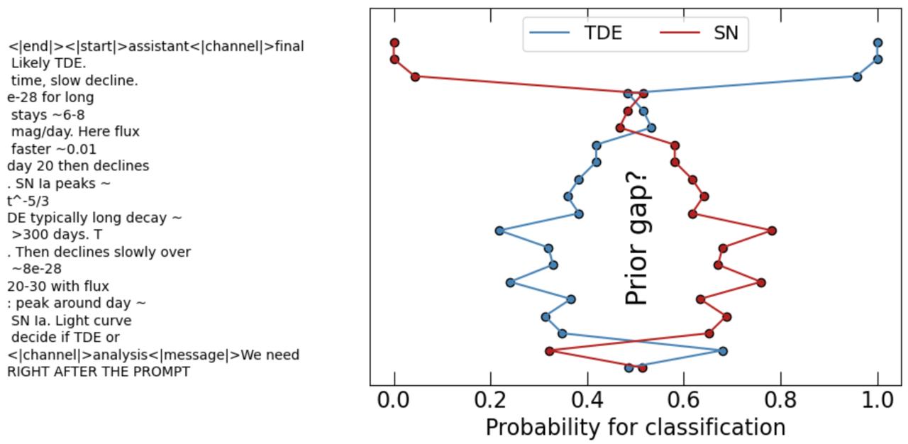
FINAL_HDR every five tokens in the Chain of Thought, effectively asking the model: “If you must decide now, what is your classification?” This shows that once the model understands the task, it initially assigns higher probability to "SN".
The natural next question is whether this is a one-off effect or a consistent pattern across many objects. The larger-sample result, shown in Figure 3, suggests that it is indeed a recurring trend.
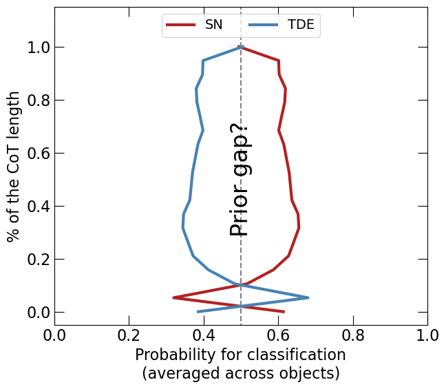
FINAL_HDR every five tokens in the Chain of Thought. The y-axis is rescaled so that all trajectories are aligned.
This is what made me think of a prior gap. We know from the astrophysical literature that SNe are much more common than TDEs. If I had to guess the label of a random transient without looking at the data, I would almost always guess SN. That is exactly what a prior is: a preference before fully digesting the evidence.
So one possible interpretation is that the model begins with an SN prior, and only later updates away from it once enough evidence accumulates.
Still, I do not think this interpretation is fully settled, and there are at least a few alternative explanations.
First, there is likely a training-distribution effect. SNe have been studied for decades and are much more prevalent in the literature and in scientific text than TDEs. TDEs, while predicted much earlier, only became a major observational topic relatively recently. So even before we talk about the prompt, there is every reason to expect class imbalance in pretraining data.
Second, the tokenization itself may matter. The fact that "SN" is a single token while "TDE" is split across two tokens could itself produce a systematic asymmetry in sequence probability. In that case, part of what I am calling a “prior gap” may actually be a readout artifact introduced by the tokenizer.
Third, the prompt framing could have introduced some bias. To test this, I swapped the order of the words "SN" and "TDE" in the prompt and reran a few experiments. The main trend remained: the model still tended to prefer "SN" early and only later shift toward "TDE" when the evidence became strong enough.
So at this point, my interpretation is not that I have literally identified the prior inside the model. Rather, I think I have identified a robust prior-like early preference that behaves in a very Bayesian way: the model starts from a default leaning toward the more common class and only later revises that leaning once the evidence accumulates.
Closing remarks
What I find most interesting here is not just that few-shot prompting improves performance, but that it seems to do so in a way that resembles evidence accumulation against an initial default guess. In that sense, the model behaves as if it starts from a prior over classes and then updates that prior as the Chain of Thought unfolds. I do not think this post proves that LLMs implement Bayesian inference in any literal sense, but I do think that Bayesian language is useful here. It gives us a concrete way to talk about bias, updates, and evidence in a framework that is both intuitive and testable.
References
[1] Brown et al. 2020, arXiv:2005.14165